If you want to do all of the following steps on your own, you can download VLOOKUP example Excel sheet. We will use the same Excel sheet for the following tutorial.
What is VLOOKUP?
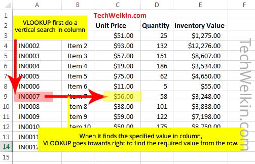
VLOOKUP is an Excel function that searches for values in a specified column. In a spreadsheet, columns are vertical. This is why the column search function is called VLOOKUP or Vertical Lookup. Using VLOOKUP, you can tell Microsoft Excel (or other spreadsheet like Google Sheets) that you are looking for a specific value in a given column. The function will find the row where the specified value is present. Once the row is located, the function can retrieve other values in that row.
Example of VLOOKUP
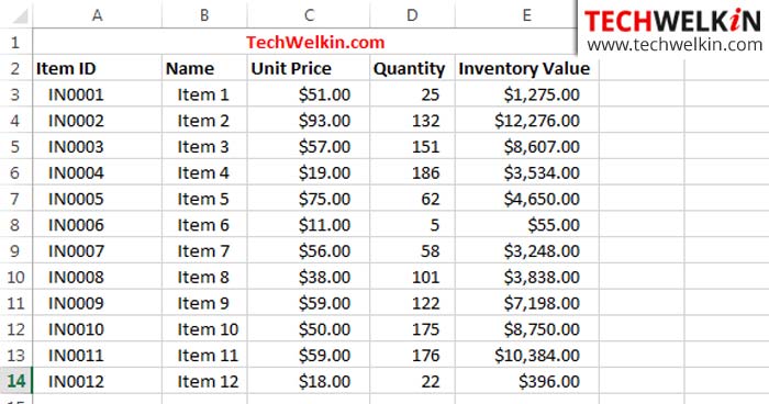
We will use the following Excel sheet to demonstrate the functioning of VLOOKUP. This sheet contains sample data of an inventory. Now let’s assume that you want to know the unit price of the item whose Item ID is IN0007. How would you do this? VLOOKUP can easily answer this question. Looking at the above Excel sheet, it is easy to find the unit price of any item, so you may wonder why do you need a special function for this? Well, the above given sheet contains a small amount of data. But what if the spreadsheet contains thousands of rows? This function can help you in such situations. Now let’s see how VLOOKUP works and how it can answer the above question.
VLOOKUP Tutorial
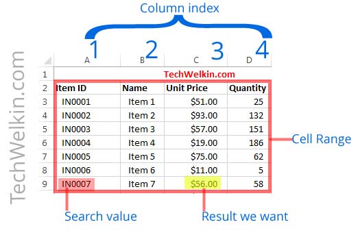
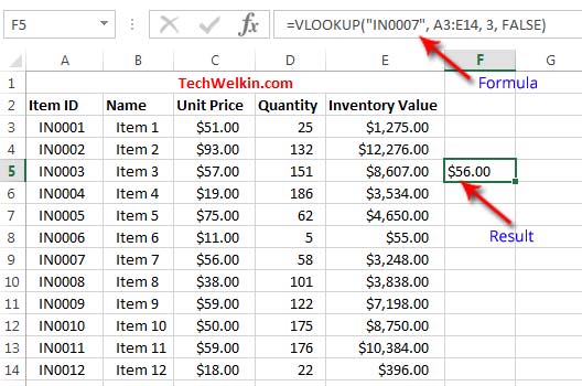
We know that VLOOKUP is an Excel function. So, we begin in the same way as we write all other formulas in Excel. First place your cursor in a cell where you want the result to appear. For example, we put the cursor in cell F5. Now, to begin the formula, type equal to sign ( = ) in the cell and then type VLOOKUP and begin the brackets for writing the parameters: =VLOOKUP( Parameters of VLOOKUP function are: Now because we want to base our search on Item ID IN0007, so we type this value as first parameter: =VLOOKUP(“IN0007” NOTE: The value that you want to look up must exist in the first column of the cell range that you will specify in the second parameter. What it actually means is that VLOOKUP will search for the given value only in the first column of the range. For example, if you want to search in the range A3:E14, then the look up value must be in column A. If the look up value is in column B, then you have to start cell range from column B (something like B3:E14). In second parameter, we need to tell VLOOKUP about the cell range in which we want to make this search. We will search the entire data in our example, therefore the cell range would be A3:E14 =VLOOKUP(“IN0007”, A3:E14 So far so good! isn’t it? Now we inform the function about what we want as result. In third parameter, we need to tell the function about the column index in which the result is located. We want to know the unit price and the column index of the unit price is 3. It is intuitive; column A has index 1, column B has index 2… and so on: =VLOOKUP(“IN0007”, A3:E14, 3 NOTE: Column index must be counted only for the columns in range. For example, if range is B2:E14, then column B becomes column 1. Therefore, in this context, column A is not always number 1. In the end, we tell the VLOOKUP function that we want precise result and that the function should not do any approximation. This fourth parameter is optional and it can either be TRUE or FALSE. If you do not specify anything as fourth parameter, the default value will be TRUE. NOTE: If you specify TRUE, then the function will assume that the first column (i.e. the look up column) in the cell range is sorted either numerically or alphabetically. The approximate search will attempt to find the closest value going from top to bottom. Therefore, this option is useful mostly if you’re searching for numerical values. It can answer questions like which item has quantity equal to or closest to 100. We don’t want to do any approximation, so we explicitly use FALSE as the fourth parameter: =VLOOKUP(“IN0007”, A3:E14, 3, FALSE That’s it! Now close the bracket. The complete formula should look like: =VLOOKUP(“IN0007”, A3:E14, 3, FALSE) You’re done! It’s time to hit the ENTER key and see the results. Wasn’t it easy? If you followed all the steps, we are sure that you learned everything. We also recommend that you try and understand all the parameters. Once you’ve understood how the function works, you will not face any problem. To help you even further, here are some more examples for you to test.
More Examples of VLOOKUP
Based upon the example sheet that we have given, let’s consider a few more examples of the VLOOKUP function. These examples demonstrate the ways in which this function can be useful. =VLOOKUP(175, D3:E14, 2, FALSE) The above formula finds the inventory value where quantity is 175. This example will show $8,750.00 as result. Here, you should note that we have used a cell range that starts from column D. Consequently, column D bears the index 1 and we count the index number accordingly. =IF(VLOOKUP(“IN0007″,A3:E14,4,FALSE)>50,”Enough Stock”,”Reorder”) The above example, combines VLOOKUP function with IF function. It will return Enough Stock if the quantity for item ID IN0007 is greater than 50. If quantity turns out to be less than 50, the function will return Reorder. Here we see how VLOOKUP can be combined with other functions to answer more complex queries.
Errors in VLOOKUP
When you use VLOOKUP, sometimes you encounter errors. In this section, we are explaining some of the common VLOOKUP errors.
#N/A error in cell
You get this error when VLOOKUP isn’t able to find a matching look up value. If you have set approximation as TRUE then chances are that you have asked VLOOKUP to find a value which is smaller than the smallest value in the column. For example, in our datasheet, if you use the following: =VLOOKUP(3, D3:E14, 2, TRUE) You’ll get #N/A error because the smallest value in the quantity column is 5 and you’re asking VLOOKUP to find 3. If you keep approximation to FALSE and you get #N/A error, then the simple reason is that VLOOKUP could not find the look up value you asked for. For example, =VLOOKUP(100, D3:E14, 2, FALSE) will throw #N/A error because the value 100 does not exist in the quantity column.
#REF error in cell
#REF error occurs when you specify column index higher than the number of columns in the cell range. For example: =VLOOKUP(100, D3:E14, 3, FALSE) will throw #REF error because total number of columns in the specified cell range is 2 and you’re trying to refer to the column with index 3.
#VALUE! error in cell
The #VALUE! error is encountered when number of columns in cell range is less than 1
#NAME? error in cell
This error comes when you do not enclose the look up value in quotes. If your looking up for a string value, e.g. a name, then you should enclose it in quotes. However, if look up value is a number, for example quantity, then double quotes should not be used. The following example will throw #NAME? error: =VLOOKUP(Item, A3:E14, 3, FALSE) To get rid of the #NAME? error you just need to enclose the item name in double quotes. In the end, we present the following video tutorial for those who prefer to learn by watching!
We hope that this tutorial on VLOOKUP function of Excel was helpful for you. Please feel free to ask if you have any questions related with this subject. We will do our best to assist you. Thank you for using TechWelkin! Comment * Name * Email * Website
Δ